ESLII-Chap2 监督学习概述

摘要 ESLII(The Element of Statistical Learning, Second Edition)是统计学习的经典之作。作为一枚学渣,博主读ESLII很费力,最近每天晚上有空就会读,但每次只能肯得动几页。同时,对于里面的一些算法或者例子也会自己用Python 实现一遍以加深理解,也能练习学习一下Python。这篇是ESLII第二章一些总结。


基本概念、术语与标记

统计学习又称统计机器学习,是关于计算机基于数据构建概率统计模型并运用模型对数据进行预测与分析的一种学科。监督学习(Supervised Learning)是统计机器学习中应用最为广泛的一种,监督学习通过已有的训练样本,即已知输入以及其对应的输出,在某个评价准则下去训练得到一个最优模型,再利用这个模型将新的输入映射为相应的输出。

在统计文献中,输入(input)又被称为自变量(independent variable)或预测变量(predictor),在模式识别文献中,也被称为特征(feature);输出(ouput)又被称之为因变量(dependent variable)或者目标变量(target variable)或者响应(response)。在ESLII中,这些命名经常交替使用。

在ESLII中,各种术语通常使用以下约定好的标记方法:

  • 大写字母,标量或向量,通常代表某个变量(输入变量或者输出变量):
    • $X$ - 输入变量; 当$X$为向量时,$X_j$是$X$的第$j$个分量;
    • $Y$ - 输出类型为定量变量(Quantitative Output variable);
    • $G​$ - 输出类型为定性变量(Qualitative Output variable)。
  • 小写字母,标量或向量,表示某次的观测变量,例如$x_i$为变量$X$的第$i$次观测变量;
  • 黑体大写字母,矩阵,例如$\mathbf{X}$为$N \times p$矩阵,表示$N$次观测变量$x_i$。

通常,向量不用黑体表示,除非该向量具有$N$项,例如$\mathbf{x}_j$代表$X_j$的$N$观测值,而$x_j$代表$X$的一次观测值。另外常用的变量还有:

  • $K$ - 因变量的取值集合的元素,即$K=\text{card}(G)$;
  • $p$ - 自变量或预测变量的分量个数;
  • $N$ - 观测次数。

两种简单的监督学习算法

范例:二维分类问题

以二维平面的分类问题为例,引入两种简单的监督学习算法:最小二乘算法(Least Squares,LS)以及最邻近算法(Nearest-Neighbor Method)。下图参照ESLII Figure2.1的场景2进行随机生成,即二维平面的样点被分为blue(数值0)和orange(数值1)两类,且每一类各由10个服从高斯分布的变量构成。
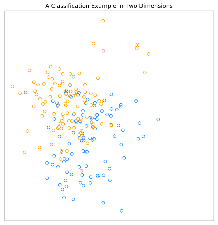
二维分类范例

该图的Python实现如下:

1
2
3
4
5
6
7
8
9
10
11
12
13
14
15
16
17
18
19
20
21
22
23
24
25
26
27
28
# IPython3 
import numpy as np
import matplotlib.pylab as plt
%matplotlib inline

def gen_data(mean, cov, n_gauss, n_observ):
mean_gauss = np.random.multivariate_normal(mean,cov,n_gauss)
#print(mean_gauss)
data = mean_gauss[np.random.randint(0,n_gauss,n_observ)] + np.random.multivariate_normal([0,0],cov/5,n_observ)
return data

# training samples
data_bule = gen_data([1,0],np.eye(2)/1,10,100)
data_orange = gen_data([0,1],np.eye(2)/1,10,100)

# set the figure parameters
plt.figure(figsize=(8,8),dpi=120) # dpi 300 for printing; 72 or 120 for web display
plt.tick_params(left='off',bottom='off',labelleft='off',labelbottom='off')
plt.title("A Classification Example in Two Dimensions")

# plot the training samples
plt.scatter(data_bule[:,0],data_bule[:,1],marker='o',edgecolors='dodgerblue',color='none')
plt.scatter(data_orange[:,0],data_orange[:,1],marker='o',edgecolors='orange',color='none')

# square the figure
plt.axis('square')

plt.show

线性模型以及最小二乘

第一类分类方式是根据线性模型采用最小二乘算法进行分类。该方法的模型、评价准则以及算法如下:

模型 (向量表示法):

其中,$X^T = (1, X_1, X_2,…,X_p)$。

在 $(p+1)​$-输入输出空间中, $(X,\hat{Y})​$ 代表一个超平面(hyperplane);如果$X​$中包括常量$X_0 = 1​$,则该超平面包含原点,属于一个子空间;如果$X​$中不包括常量$X_0 = 1​$,则该超平面输入仿射集(affine set)。

准则(最小残差平方和):

可用矩阵形似表示为:

算法:

然后,根据该模型对第$i$对测试数据$x_i$的输出为:

最终,$x_i$的分类结果为:如果$\hat{y}>0.5$,$ \hat{G}$=orange,否则$ \hat{G}$ = blue

下图为采用上述方法进行分类的结果。其中,图中的标记为‘o’为点输入的训练数据,其颜色为所属类别,标记为’.’为输入的测试数据,其颜色代表所属类别,黑色实线为判决边界的一段。

LS分类

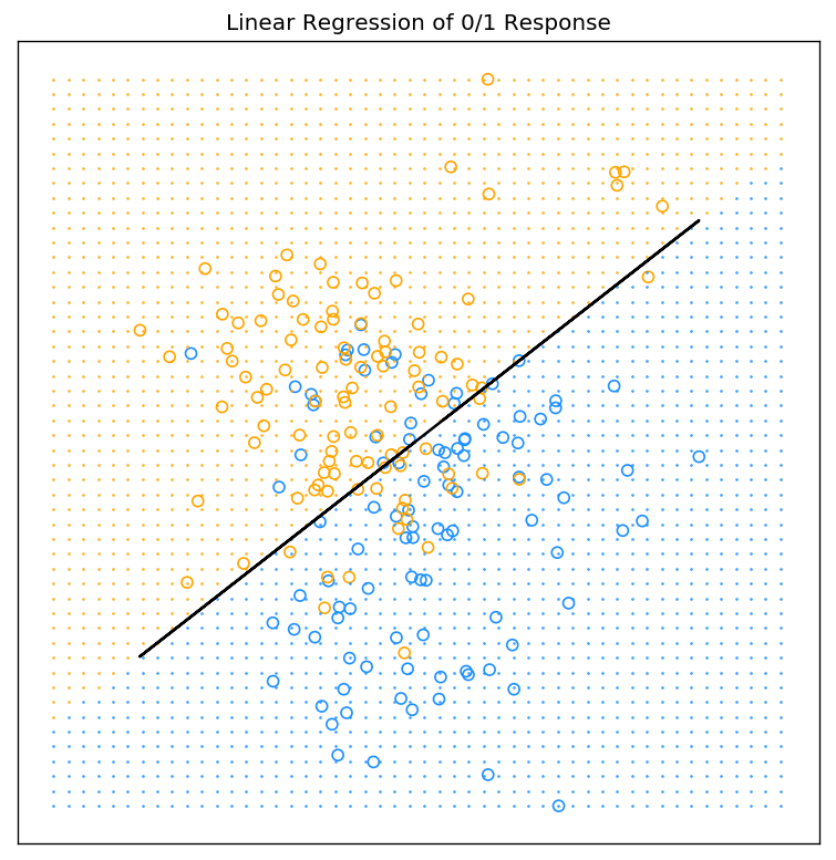
最小二乘算法以及上图的Python代码(上个代码片段的后续)如下:

1
2
3
4
5
6
7
8
9
10
11
12
13
14
15
16
17
18
19
20
21
22
23
24
25
26
27
28
29
30
31
32
33
34
35
36
37
38
39
40
41
42
## LEAST SQUARES##
X = np.vstack((data_bule, data_orange))
X = np.hstack((np.ones((200,1)),X))
Y = np.ones((100,1))*np.arange(2)
Y = np.reshape(Y,(200,1),order='F')

# parameters of least squares algorithm
beta = np.dot(np.dot(np.linalg.inv(np.dot(X.transpose(),X)),X.transpose()),Y)


# test samples
v = np.linspace(X.min(),X.max(),50)
xn1,xn2 = np.meshgrid(v,v)

# output of new test samples
yn = (beta[0]+beta[1]*xn1+beta[2]*xn2)>0.5
# decision boundary {x: x^T*beta = 0.5}
x2 = X[:,2].reshape((200,1))+(0.5-np.dot(X,beta))/beta[-1]


# set the figure parameters
plt.figure(figsize=(8,8),dpi=120) # dpi 300 for printing; 72 or 120 for web display
plt.tick_params(left='off',bottom='off',labelleft='off',labelbottom='off')
plt.title("Linear Regression of 0/1 Response")

# plot the training samples
plt.scatter(data_bule[:,0],data_bule[:,1],marker='o',edgecolors='dodgerblue',color='none')
plt.scatter(data_orange[:,0],data_orange[:,1],marker='o',edgecolors='orange',color='none')

# plot the test samples
plt.plot(xn1[yn==True],xn2[yn==True],linestyle='none',marker='.',markersize=1,color='orange')
plt.plot(xn1[yn==False],xn2[yn==False],linestyle='none',marker='.',markersize=1,color='dodgerblue')

# square the figure
plt.xlim([X.min(),X.max()])
plt.ylim([X.min(),X.max()])
plt.axis('square')

# plot the decision boundary
plt.plot(X[:,1],x2,color='black')

plt.show

最邻近算法

最邻近算法利用训练集合$\mathcal{T}$中距离输入变量$x$最近的$k$的观测值去计算$\hat{Y}$:

其中,$N_k(x)$是$x$在训练集合中的最邻近集合;k为最邻近算法的参数,代表临近集合中的样本个数,即。最后,若$\hat{Y}$>0.5,则判决为orange,否则为blue。下图为采用最邻近算法的分类结果,其中,图中的标记为’o’为点输入的训练数据,其颜色为所属类别,标记为’.’为输入的测试数据,其颜色代表所属类别。

knn分类

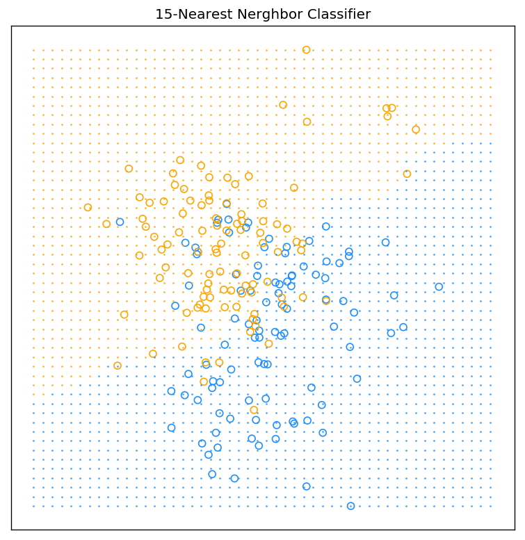
最邻近算法以及上图的Python代码(上个代码片段的后续)如下:

1
2
3
4
5
6
7
8
9
10
11
12
13
14
15
16
17
18
19
20
21
22
23
24
25
26
27
28
29
30
31
32
33
34
35
36
37
38
39
40
41
42
43
44
45
46
47
48
49
50
def knn_classify(test_sample, training_sample, training_sample_resp, k):
# test_sample: the samples for test
# training_sample: the samples used for training
# training_sample_resp: the respone of the training samples
# k: parameters of KNN method

n = test_sample.shape[0]
p = test_sample.shape[1]
# calc the neighbors
distance_array = np.linalg.norm(test_sample.reshape((n,1,p))-training_sample,ord = 2, axis = 2) # broadcasting,and calculate the norm
index_neighbor = np.argsort(distance_array)[:,0:k]
neighbor = training_sample_resp[index_neighbor]
# apply KNN fit
test_sample_resp = np.sum(neighbor,axis=-2)/k
# decision
resp_set = np.unique(training_sample_resp)
l = resp_set.size
test_sample_resp = resp_set[np.argsort(np.abs(test_sample_resp-resp_set.reshape((l,))))[:,0]]

return test_sample_resp

##
test_sample = np.hstack((xn1.reshape((xn1.size,1)),xn2.reshape(xn2.size,1)))
training_sample = np.vstack((data_bule,data_orange))
training_sample_resp = np.ones((100,1))*np.arange(2)
training_sample_resp = np.reshape(training_sample_resp,(200,1),order='F')

test_sample_resp = knn_classify(test_sample, training_sample, training_sample_resp, 15)

# set the figure parameters
plt.figure(figsize=(8,8),dpi=120) # dpi 300 for printing; 72 or 120 for web display
plt.tick_params(left='off',bottom='off',labelleft='off',labelbottom='off')
plt.title("15-Nearest Nerghbor Classifier")

# plot the training samples
plt.scatter(data_bule[:,0],data_bule[:,1],marker='o',edgecolors='dodgerblue',color='none')
plt.scatter(data_orange[:,0],data_orange[:,1],marker='o',edgecolors='orange',color='none')

# plot the test samples
plt.plot(test_sample[test_sample_resp==1,0],test_sample[test_sample_resp==1,1],linestyle='none',marker='.',markersize=1,color='orange')
plt.plot(test_sample[test_sample_resp==0,0],test_sample[test_sample_resp==0,1],linestyle='none',marker='.',markersize=1,color='dodgerblue')

# square the figure
plt.xlim([X.min(),X.max()])
plt.ylim([X.min(),X.max()])
plt.axis('square')

# plot the decision boundary

plt.show

注:

  • 为了代码的高效简洁,采用了Python的Broadcasting机制。关于Broadcasting的更多详细信息点击参考这里
  • 博主目前还不会绘制ESLII Figure2.2中KNN算法的判决边界,但是通过观察上图中’.’表示的区域可以大致勾勒出KNN算法的判决边界为一条或者多条的曲线;
  • 当训练样本增多时,本篇文章里介绍的LS算法和KNN算法的复杂度将急剧的增加;在后续的文章中,我们将采用QR分解来解决LS算法的矩阵求逆过程;采用KD树的方法来解决KNN算法的搜索过程。

从最小二乘到最邻近算法

  • 最小二乘算法假定输入输出符合线性模型,进而判决边界光滑;最邻近算法不对输入输出做任何假设,进而其判决边界受到训练样本的影响;
  • 最小二乘算法相比最邻近算法具有低方差高偏置(low variance and high bias: stable)的特点。

统计决策理论

统计决策理论(statistical decision theory)使用训练样本信息以及样本信息之外的其他信息(损失函数以及先验信息)来形成决策过程。

下面用统计决策理论的角度去分析最小二乘和最邻近算法。这两个算法均选择损失函数(loss function)为$L(Y,f(X))=(Y-f(X))^2$,则选择模型$f$的准则为最小化均方预测误差(expected squared predication error, EPE):

根据上述准则的$f(x)$为:

上述方程又被称之为回归方程(regression function),即当评价准则为均方误差时,$Y$在$X=x$处的最佳估计为$Y$的条件期望。

  • 最小二乘和最邻近算法本质上是用训练样本去估算该条件期望:
    • 线性模型$f(x)\approx x^T\beta$的统计决策解为$\beta=[\mathbf{E}(XX^T)]^{-1}\mathbf{E}(XY)$ ;
    • 最小二乘算法将求期望(自相关和互相关)的运算用全部样本求平均的方法替代;
    • 最邻近算法同样将期望松弛为样本数据的平均,且将$X=x$的条件松弛为$x$附近的邻域。
  • 虽然近似方法相似,但两者选择模型不同:
    • 最小二乘算法假定$f(x)$是线性模型;
    • 最邻近算法假定$f(x)$在$X=x$足够小的邻域内保持常数。

当统计决策的损失函数由二阶的均方误差替换为一阶的$\mathbf{E}|Y-f(x)|$,则最小化该损失函数的$f(x)$为:

当输出变量为定性变量$G\in \mathcal{G}$时,损失函数通常定义为$K\times K$的矩阵$L$,其中$K=\text{card}(G)$。$L(k,l)$为将$\mathcal{G}_k$的变量分类为$\mathcal{G}_l$的代价。此时最小化损失函数的决策函数$\hat{G}(x)$为:

以上方程又被称之为贝叶斯分类器(Bayes classifier)